Why does ensemble model work better than individual model?

A single model is known to make errors. If we make classifiers that make different errors, the misclassified examples will not be the same. Thus, the models can complement each other, and the error can be reduced. So, instead of training one model for the given problem, we can train multiple of them.

• Ensemble Models
• Bagging
• Variance of the Ensemble Model
• Random Forests
• Appendix

Ensemble Models

Till now, we have seen training individual hypothesis function (also known as model) for classification/regression tasks. A single model is known to make errors. If we make classifiers that make different errors, the misclassified examples will not be the same. Thus, the models can complement each other, and the error can be reduced. So, instead of training one model for the given problem, we can train multiple of them.

Moreover, individual models suffer from high variance. Different training data gives different splits which leads to different results. In the bias-variance decomposition of the test error, the variance term has the aggregated hypothesis/average hypothesis. The variance measures the deviation between this average hypothesis and the hypothesis trained on a particular dataset. To reduce the variance, we must ensure that the hypothesis trained on a single data set is close to the average hypothesis.

Theoretically, we can train multiple models on different datasets, and aggregate their results. And it can be shown that the error from this aggregated model will be lesser compared to training an individual model because of the fact that the ensemble models have less variance. In practice, we are given only one dataset. We don’t have multiple datasets to train multiple classifiers. To overcome this, in ensemble methods, we create multiple datasets by sampling with replacement.

The individual models that go into ensemble do not need to be very good; they just have to be better than chance. Thus, every individual component of an ensemble is called a weak learner. As long as they are better than chance, the ensembles are always guaranteed to give dramatic improvements in performance by reducing the variance of the model compared to individual classifier.

But how do we construct models that make different errors, and thus complement each other? There are two ways of doing ensembling: Bagging and Boosting.

Bagging

Bagging stands for Bootstrap Aggregation. In bagging, we simply sample the given training data with replacement to create multiple datasets (called as bootstrap samples) and train multiple classifiers to create an ensemble. Suppose the dataset $D = {x_1, \dots, x_N}$ contain $N$ samples. We create $B$ training sets by sampling with replacement so that each new dataset $D_b$ has $N$ samples.

• The probability of a sample $x_i$ being picked in one draw is $\frac{1}{N}$.
• The probability of a sample $x_i$ being picked in one draw is $1-\frac{1}{N}$.

Since $N$ draws are independent (because of replacement), the probability of $x_i$ never appears in $D_b$ is $ \left( 1-\frac{1}{N} \right)^N$. As $N \to \infty$,

So approximately, $P(x_i \notin D_b) \approx \frac{1}{e} \approx 0.368$. This is the famous bootstrap result:

• In each bootstrap sample, roughly 36.8% of the original samples are left-out. Equivalently, about 63.2% of unique original samples appear at least once. This brings an implicit regularization effect; because it creates an implicit validation data.

Now, we have $b=1, \dots, B$ datasets each of size $N$. We train $B$ independent classifiers: $h_1(x), h_2(x), \dots, h_B(x)$. The models can be trained independently and in parallel. The final prediction is

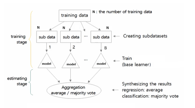
In the inference stage, a test data point $x$ is fed into the trained models. We get prediction from all these $B$ models. We then combine the results from all the classifiers by taking average (in case of regression or if the classifiers output probability), majority vote (in case of classification). Every classifier has a similar weight towards the final prediction.

The injected randomness in the dataset creation process results in uncorrelated models (not identical models) which when combined improve the overall model generalization.

Variance of the Ensemble Model

The primary objective of ensembling is to reduce the variance of the model so that the overall error associated with the model can be reduced.

Let $x$ be a fixed data point, and the $i$th hypothesis (model) is $h_i$. Suppose $z_i$ represents a random variable corresponding to the prediction of the $i$th hypothesis on a given data point. Then,

Because the training set used to build $h_i$ is random (e.g., a bootstrap sample), $h_i$ itself is random, and therefore $z_i$ is a random variable. Suppose the original dataset is $ {x_1, x_2, x_3 }$. Possible bootstrap samples include

• ${x_1, x_1, x_1 }$
• ${x_1, x_2, x_1 }$
• ${x_2, x_2, x_1 }$, etc.

There are $3^3 = 27$ possible ordered samples, and each has an equal probability of $\left(\frac{1}{3} \right)^3 = \frac{1}{27}$ to be selected. In general, probability of getting a particular ordered bootstrap sample is $\left(\frac{1}{N} \right)^N$. We get bootstrap samples $D_1, \dots, D_B$ and train $h_1, \dots, h_B$ models. That is,

1. We draw a bootstrap sample from the given training data
2. Train a model using the same algorithm and hyperparameters
3. Evaluate at $x$

Suppose we repeatedly do this process many times, then the prediction of the first model $h_1$ at $x$ would vary depending on which bootstrap sample it received. Thus,

has a probability distribution. We have $B$ such random variables, $z_1, \dots, z_B$, because we have $B$ models trained.

Since every hypothesis function is trained on the data sampled from the same distribution, the distribution of its prediction at $x$ will be the same. That is, $z_1, \dots, z_B$ are identically distributed. But note that they are not independent because we have bootstrap samples that overlap. When we do random sampling with replacement and create multiple datasets, our i.i.d assumption across these data sets will be broken. The created data sets will overlap with each other. As they overlap, the resulting models are usually correlated. That is, the prediction (or the error) made by one model is correlated with the prediction (or the error) made by another model.

So, we say that $z_1, \dots, z_B$ are identically distributed but correlated, which can be formulated as:

$\rho$ denotes the correlation between individual models. We know that

From the definition of ensemble, we have

Then, the variance of the ensemble is:

There are $B$ number of $z_i$’s. So, there are $B(B-1)$ ways to select an ordered pair. Then,

Define:

We want $A \leq 1$ so that the variance of the ensemble is less than or equal to the variance of the individual model. $A$ can be rewritten as:

Then

We want $1-A \geq 0$, i.e., we want both the RHS terms to be $\geq 0$.

• Since $B \geq 1$, $\left( 1- \frac{1}{B} \right)$ is always $\geq 0$.
• The correlation coefficient $\rho$ satisfies $\leq 1$, so $(1- \rho)$ is always $\geq 0$.

which implies $1-A \geq 0 \implies A \leq 1$.

When do we get equality?

There are two cases in which this can happen:

• When $B=1$: no ensemble, then $\text{var}(\bar{z}) = \sigma^2$ (same as the variance of the individual classifier). Or,
• When $\rho=1$: all models are perfectly correlated. That is, when all the models are built using the same data, same algorithm and the same hyperparameters. Averaging identical models gives no variance reduction.

When is the variance strictly smaller?

Whenever $B > 1$ and $\rho < 1$, then $\text{var}(\bar{z}) < \sigma^2$. This is the proof that ensembling always reduces the variance of the model, thus reducing the overall error of the model.

To reduce $\text{var}(\bar{z})$, we should either:

1. Increase $B$ - increase the number of models
2. Decrease $\rho$ - decrease the correlation among the models. That is, we need to ensure that the individual models are uncorrelated.

The higher the number of models we ensemble, the lower the variance. Then, can’t we just add as many models as possible into our ensemble to reduce the variance as much as possible? As $B \to \infty$, the variance of the ensemble tends to $\text{var}(\bar{z}) \to \rho \sigma^2$. That is, even with infinitely many models, the variance cannot go below $\rho \sigma^2$. The residual variance is due to the correlation among the models.

Simply increasing the number of models $B$ increases the correlation $\rho$ among the models, that is, the predictions of the individual models become more correlated. So, we need to increase $B$ but also reduce $\rho$. There are various ways to reduce $\rho$. The Random Forests algorithm uses one of those techniques.

Random Forests

The classical example of an ensemble model that uses bagging technique is Random Forests. In Random Forests, the individual models are decision trees, and it can be used for both classification and regression.

The randomness injected into the dataset creation process to generate bootstrap samples ensures that the individual trees are distinct from one another. In addition to it, at each node of every tree, the best split point is found based on a random subset of the features. How does this ensure that the resulting trees are uncorrelated?

In practice, there will be a small set of strong predictors of the target and multiple moderate predictor variables. Every time we build a tree, the same features dominate the top nodes. In such cases, all the resulting trees look the same, and the predictions from those trees will be correlated. Random feature subsampling helps us avoid this and build trees with different features.

Random forest uses deep decision trees (without pruning), but it is less prone to overfitting because it uses the sampled (row and column-sampled) data and averages the results from multiple trees. Thus, pruning is not necessary.

Say we have a training dataset with $N$ observations and $p$ features. This training data is sampled both row-wise and column-wise in random forest.

• First, with replacement, we sample $N$ rows.
• We then build a tree on this data. At each node of the tree, we do column sampling from the total of $p$ features (without replacement). The number of features to be selected at every node is considered a hyperparameter. By a rule of thumb, the number of features to sample, $m$, can be calculated as $m=\sqrt{p}$ or $m = \log_2(p)$.

These two randomness ensures that the predictions from individual models are different, and the trees are uncorrelated.

Appendix

We have

We saw the upper bound for $A$, which is, $A \leq 1$. But what if $A$ is negative? For example, if $B=10$ and $\rho=-1$, then $A = \frac{1}{10} + \left(1-\frac{1}{10} \right) (-1) = -\frac{8}{10}$. In that case, the variance of the ensemble is negative, which is not possible. So, where is the catch? What ensures that $A \geq 0$?

The resolution is that not every value of $\rho \in [−1,1]$ is actually possible when we have $B$ identically distributed random variables with the same pairwise correlation.

We know that the covariance matrix is always positive semidefinite. That is, it must have non-negative eigenvalues. The covariance matrix of the random variables $(z_1, \dots, z_B)$ is

The eigenvalues of this matrix are $\sigma^2 (1-\rho)$ with multiplicity $(B-1)$ and $\sigma^2 (1 + (B-1)\rho)$ with multiplicity 1. Therefore, we must have

and

And we have

The numerator term $(B-1)\rho + 1\geq 0$ implies that $A \geq 0$. And the true admissible range for $\rho$ is