Wasserstein Convergence of SGMs

Can we establish upper convergence bounds for Score-based Generative Models under Semiconvexity and Discontinuous Gradient conditions? The paper titled “Wasserstein Convergence of Score-based Generative Models under Semiconvexity and Discontinuous Gradients” by Bruno and Sabanis (2025) addresses this question. This article provides the detailed derivation of one of the results from this paper.

• Abstract
• Background
• Wasserstein Convergence Analysis of SGMs
  • Upper bound on $W_2\left(q_T, \tilde{p}_T\right)$:
• Final Result
• References

Abstract

Most convergence proofs in Score-based Generative Models (SGMs) such as de-noising score matching and diffusion models assume ideal settings:

• The energy function $f$ of the target distribution is $\mu$- strongly convex.
• The score function (the gradient of the log density) is Lipschitz continuous.

The Langevin diffusion algorithm converges to the target $p^*$ for any distribution, but the rate of convergence happens at an acceptable rate when the energy function $f$ of the target distribution is $\mu$- strongly convex. Such conditions are rarely satisfied in practice, and doesn’t truly reflect the complexity of the real data.

In this paper, the authors have relaxed these assumptions and have established convergence guarantees for SGMs targeting semi-convex distributions with potentially discontinuous gradients in terms of the Wasserstein-2 distance. They have established explicit, dimension and parameter dependent, non-asymptotic Wasserstein-2 convergence upper bounds under these relaxed assumptions.

Background

The core idea behind diffusion models is:

Forward process:

We are given samples from some distribution $p^*$. We add noise to these samples until its distribution becomes pure Gaussian noise.

Let $(X_t)$ be the forward process where $t\in [0,T]$ and $X_0 \sim p^*$. The Langevin diffusion process with the source distribution $p^*$ and the target the pure Gaussian noise $\mathcal{N}(0, I)$ is characterized by:

where $W_t$ is the Weiner process.

Reverse Process:

We start with noise and transform it back to the target distribution by estimating the score function of the forward process.

Let $(Y_t)$ be the reverse process where $t\in [0,T]$. And it should be

The reverse process can also be characterized by a SDE:

where $p_t = p(X_t)$.

Ideally $Y_0 \sim p(X_T)$. But in practice, the initial distribution is taken to be the standard Gaussian distribution, $\mathcal{N}(0, I)$. As a result, the backward process becomes:

Since the target distribution $p^*$ is unknown, the score function $\nabla \log p_t$ cannot be computed exactly. We learn an estimator $s$ that approximates the score of the forward process over a fixed time window $[0,T]$. On incorporating this approximation, the process is:

In practice, we discretize the process. Let $\gamma \in (0,1)$ be the step size for time steps $j=1, \dots, J$. Then the EM approximation of the reverse process is:

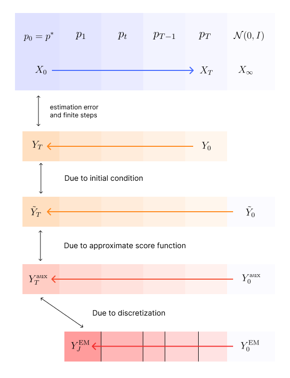
This breaks down the deviation between the final distribution of the EM approximation and the target distribution into four components. From the bottom of the figure,

• The first component is the deviation between the EM approximation and the auxiliary process, which is due to the discretization error.
• The second component is the deviation between the auxiliary process and the backward process, which is due to the score estimation error.
• The third component is the deviation between the backward process that starts from the standard Gaussian and the backward process that starts from the final distribution of the forward process. This is due to the difference in their initial distributions.
• The fourth component is the deviation due to estimation error and finite number of steps in the backward process in practice.

Wasserstein Convergence Analysis of SGMs

Since we are measuring the deviation in terms of a distance, then using the triangle inequality, we can bound the deviation as follows:

Upper bound on $W_2\left(q_T, \tilde{p}_T\right)$:

Here we will derive an upper bound on the Wasserstein-2 distance between two distributions at time $T$: the distribution of the backward process that starts from the final distribution of the forward process $q_T$ and the distribution of the backward process that starts from the standard Gaussian $\tilde{p}_T$.

We know that from the definition of the Wasserstein-2 distance:

There are two diffusion processes $\tilde{Y}_t$ and $Y_t$. These processes have the same Brownian motion but different starting points.

• $Y_t$ starts from the final distribution of the forward process $p_T$.
• $\tilde{Y}_t$ starts from the invariant distribution of the forward process (the standard Gaussian)

These processes can be characterized by SDE respectively as follows:

Define a difference process

Then,

Since both processes share the same noise term $\sqrt{2} \, d\bar{W}_t$, the noise cancels out:

Let $f(Z_t) = |Z_t|^2 = \sum_i Z_{i,t}^2$ be a function of $Z_t$. Then, the change in $f$ with respect to $Z_t$ is given by

On substituting (1) and (2) and using the linearity of the inner product, i.e., $\langle a, c \cdot \mathbf{v} \rangle = c \langle a, \mathbf{v} \rangle$,

for any $t \in [0, T]$. Again, using the linearity property:

We get

On integrating over time $t$ from 0 to $T$,

On taking expectation on both the sides and interchanging the expectation and integral operators:

From Cauchy-Schwartz inequality, we know $\langle a, b \rangle \leq |a| |b|$. Let

• $a=Y_t - \tilde{Y}_t$ and
• $b = \nabla \log p_{T-t}(Y_t) - \nabla \log p_{T-t}(\tilde{Y}_t)$

Then,

Smooth Potential:

If the energy function of the target distribution $\mathcal{E}$ was $L$-smooth, then its gradient is Lipschitz continuous with constant $L$:

Using this, (4) can be written as:

Then (3) becomes

On applying the Grönwall’s Inequality, we get:

Non-smooth potential:

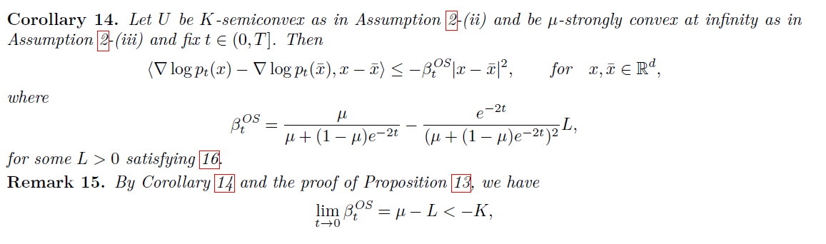
It essentially says that even if the original energy is rough, as we add noise in the forward process, the distribution $p_t$ becomes smooth over time.

• At the very start of the process ($t \approx 0$), the smoothness is governed by the underlying semi-convexity of the potential.
• As $t \to \infty $, the coefficient $\beta_t^{OS}$ would then converge to $\mu$, which represents the $\mu$-strong convexity of the distribution at infinity.

This indicates that over time, the “semi-convexity” of the original energy is completely washed away by the noise, leaving a smooth, strongly convex landscape. Using this, the third term in (3) can be written as:

Then (3) becomes:

On applying the Grönwall’s Inequality, we get:

We know the forward process SDE is:

On solving this SDE, we get:

where $m_t = e^{-t}$, $\sigma_t^2 = 1- e^{-2t}$, and $N_t \sim \mathcal{N}(0, I)$. At $t=T$,

We know that $X_T = Y_0$ and $N_T \stackrel{d}{=} \tilde{Y}_0$. On substituting,

Using the inequality $(a + b)^2 \leq 2a^2 + 2b^2$,

We know $m_T^2 = e^{-2T}$ and $(\sigma_T - 1)^2 \leq e^{-2T}$, then our final bound can be given as:

where $\mathbb{E}[|\tilde{Y}_0|^2]$ is equal to the trace of the identity covariance matrix, which is exactly $d$.

Which is of the order $O(\sqrt{d})$. The distance grows sub-linearly with the number of features or dimensions ($d$).

The estimates are explicit and exhibit the best known optimal dependencies in terms of data dimension, i.e., $O(\sqrt{d})$ in Theorem 19, and rate of convergence, i.e., $O(\gamma)$ in Theorem 21.

Final Result

For any $\delta > 0$, if we choose the parameters $\epsilon, T, \varepsilon_{SN}, \gamma$ within the range (where the values of $\epsilon_\delta, T_{\delta}, \varepsilon_{SN, \delta}, \gamma_\delta$ are given in the table 3 of the paper)

• $0 < \epsilon < \epsilon_\delta$
• $T > T_{\delta}$
• $ 0 < \varepsilon_{SN} < \varepsilon_{SN, \delta}$
• $0 < \gamma < \gamma_\delta$

It is shown that

References

1. Bruno, S., & Sabanis, S. (2025, May 6). Wasserstein Convergence of Score-based Generative Models under Semiconvexity and Discontinuous Gradients. arXiv.org. https://arxiv.org/abs/2505.03432