Energy-Based Models + LMC

We are given a set of samples from some (unknown) distribution. How can we generate more samples from this unknown distribution? In this post, we will see how to solve this problem using energy-based models and Langevin Monte Carlo (LMC) sampling algorithm.

• Problem Setup
• Solution Approach
• Loss function
• Langevin Monte Carlo
• Network Architecture
  • Training
• Inference
• References

Problem Setup

We have an underlying distribution $p^*$. We are given samples from it. Let the underlying distribution be $p^*(x)$ and the samples given are $x_1, x_2, \dots, x_m$. This forms our training set. Using only this training set (without the knowledge of $p^*$), the objective is to create more samples from $p^*$.

import numpy as np
import matplotlib.pyplot as plt
import seaborn as sns

mu = 5
sigma = 1
n_samples = 1000

# Generating samples using pseudo-random number generator
samples = np.random.normal(mu, sigma, n_samples)

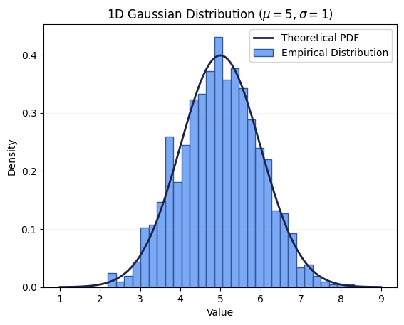
The histogram represents the data samples we actually have, while the red line represents the mathematical ideal defined by the probability density function (PDF):

Let’s pretend that we don’t know the parameters $\mu$ and $\sigma$ of the underlying distribution. We only have the samples ${x_1, x_2, \dots, x_N}$ where $N=10,000$ and $x_i \in \mathbb{R}$. How can we generate more samples from this underlying distribution?

Solution Approach

Let’s use explicit generative modelling approach to solve this problem, which is a two-step process.

1. We first learn a distribution $p$ which should be as close as possible to the underlying distribution $p^*$ (likelihood estimation problem) using the given samples. We’ll use energy-based models to learn this distribution.
2. Then, we use Langevin Monte Carlo algorithm to generate new samples from this learned distribution.

Loss function

We don’t know the form or anything about the underlying distribution. Let’s begin with parameterizing our distribution $p$ by $\theta$. Given training samples, the likelihood of those samples under our model distribution $p_{\theta}$ is:

The log-likelihood of the data is then

The objective in training is to tune $\theta$ in such a way that the log-likelihood of the data is maximized.

But we always look at the negative of log-likelihood (NLL), which is the loss:

In training, the objective is to minimize this loss. We typically use gradient descent algorithm to solve this. To use gradient descent, we need the gradient of the objective function (log-likelihood function)

\begin{equation} \nabla_{\theta} LL(\theta) = \frac{1}{N}\sum_{i=1}^N \nabla_{\theta} \log p_{\theta}(x_i) \tag{1} \end{equation}

The energy-based models assume that our distribution $p_{\theta}$ is of the form:

where $f_{\theta}(x)$ is called the energy function. The energy function takes $x$ as input and gives a real number. This can be modelled using a neural network, and $\theta$ are the parameters of this network. On substituting $p_{\theta}(x)$ in (1):

We know that

The differentiation is with respect to $\theta$. The integral is not with respect to $\theta$. So, we can just differentiate the integrand.

The gradient of the log-likelihood function for training an energy-based model can then be given by:

• The first term is the expectation of the gradient of energy with samples from $p^*(x)$.
• The second term is the expectation of the gradient of energy with samples from our learned distribution $p_{\theta}$.

At optimality, i.e., When $\nabla LL(\theta) = 0$, we must have:

Therefore, we are essentially matching the expected values of gradient of $f$ between the samples from our learned distribution and the training samples. The loss $\mathcal{L}(\theta)$ can then be given by:

This is the loss we use to train our model $f_{\theta}$.

• The first term (or LHS) can be approximated easily by the sample mean using the training samples $x_i$’s.
• The second term can be easily calculated the same way if we know samples from $p_{\theta}$.

$p_{\theta}$ is the likelihood induced by some energy-based model. How can we produce samples from it? We use Langevin Monte Carlo to generate samples from $p_{\theta}$.

Langevin Monte Carlo

We start from some initial distribution $p_0$. We can take $p_0$ to be a uniform distribution. We then apply the following update rule iteratively:

where

and $s$ is the step size and $N_k$ is a standard normal random variable. The update rule is thus given by:

We run this update rule for $K$ iterations. As $K \to \infty$, the distribution of $X_K$ converges to $p^*$, which is the distribution we want to sample from.

The LMC procedure is coded as follows:

def langevin_monte_carlo(x, model, n_steps, stepsize=None, intermediate_samples=False):
  l_samples = []
  l_samples.append(x)
  x.requires_grad = True

  for k in range(n_steps):
    if stepsize is None:
      # decaying stepsize
      current_stepsize = 1/ (k + 1)  
    else:
      # constant stepsize
      current_stepsize = stepsize    
    noise = torch.randn_like(x) * np.sqrt(current_stepsize * 2)
    out = model(x)
    grad = autograd.grad(out.sum(), x, only_inputs=True)[0]
    #Langevin step
    x = x - current_stepsize * grad + noise
    l_samples.append(x)

  if intermediate_samples:
    return l_samples
  else:
    return l_samples[-1]

Network Architecture

As we are modelling a very simple energy function $f_{\theta}: \mathbb{R} \to \mathbb{R}$, let’s just take a FFNN with only one hidden layer and LeakyReLU activation function.

class EnergyModel(nn.Module):
    def __init__(self):
        super().__init__()
        self.net = nn.Sequential(
            nn.Linear(1, 64),      # Input is 1D (batch_size, 1)
            nn.LeakyReLU(0.2),
            nn.Linear(64, 64),     # Hidden layer
            nn.LeakyReLU(0.2),
            nn.Linear(64, 1)       # Output is a single energy value
        )

    def forward(self, x):
        return self.net(x)

# Initialize and move to device
model = EnergyModel().to(device)

Training

opt = Adam(model.parameters(), lr=0.001)

for epoch in range(30):
  l_loss = []
  l_loss_mean = []
  for i, (batch_x,) in enumerate(train_loader):
        batch_x = batch_x.to(device)

        # 1. Generate 'negative' samples using the Langevin function.
        # Starting from random noise from uniform distribution
        x_fake = torch.empty(batch_x.shape).uniform_(0, 15) 
        x_fake = langevin_monte_carlo(x_fake, model, n_steps=15)

        # 2. Compute Energy scores
        energy_real = model(batch_x)
        energy_fake = model(x_fake)

        # 3. Contrastive Divergence Loss (Lower energy for real, higher for fake)
        reg_loss = (energy_real**2 + energy_fake**2).mean()
        loss = (energy_real.mean() - energy_fake.mean()) + 0.2 * reg_loss

        loss.backward()

        torch.nn.utils.clip_grad_norm_(model.parameters(), max_norm=1)
        opt.step()

        l_loss.append(loss.item())
  l_loss_mean.append(np.mean(l_loss))
  if epoch % 5 == 0:
    print(f"Epoch {epoch+1}/{30}, Loss: {np.mean(l_loss)}")

After training, the learnt energy function $f_{\theta}$ is as below:

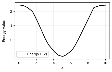
It can be observed that the energy for data points from the dataset are minimized, while the energy for randomly sampled data points are maximized.

We can then use this learned energy function to generate samples from the distribution $p_{\theta}$ using Langevin Monte Carlo. The generated samples should ideally match the underlying distribution $p^*$, which is a Gaussian distribution with mean 5 and variance 1 in our case.

Inference

Let’s begin with some initial distribution $p_0$ (say from a uniform distribution). We then apply the LMC procedure iteratively. As we run the LMC procedure for more and more iterations, the distribution of the generated samples converges to $p^*$.

x_fake = torch.empty(500,1).uniform_(0, 10)
particle_flow = langevin_monte_carlo(x_fake, model, n_steps=15, intermediate_samples=True)

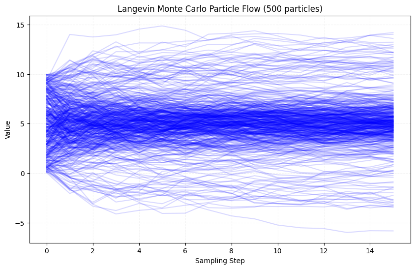
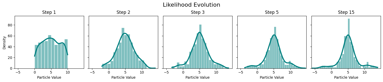
The particles start from a uniform distribution and gradually move towards the target distribution (Gaussian with mean 5 and variance 1) as we apply the LMC update iteratively. In fact, it is very fast that we can see the particles moving towards the target distribution in just a few iterations.

The generated samples can be visualized at each time step using a histogram to see how the uniform distribution is getting transformed to the target distribution.

References

1. Tutorial 8: Deep Energy-Based Generative Models — UvA DL Notebooks v1.2 documentation. (n.d.). https://uvadlc-notebooks.readthedocs.io/en/latest/tutorial_notebooks/tutorial8/Deep_Energy_Models.html

2. Swyoon. (n.d.). pytorch-energy-based-model/train_energy_based_model.py at master. GitHub. https://github.com/swyoon/pytorch-energy-based-model/tree/master