A linear regression model may overfit the training data. How can we reduce overfitting and improve generalization performance?
Model Selection
Given training data \(\{(\mathbf{x}_n, t_n)\}\) for \(n =1,2,\dots, N\) where \(\mathbf{x}_n \in \mathbb{R}^{D}, t_n \in \mathbb{R}\).
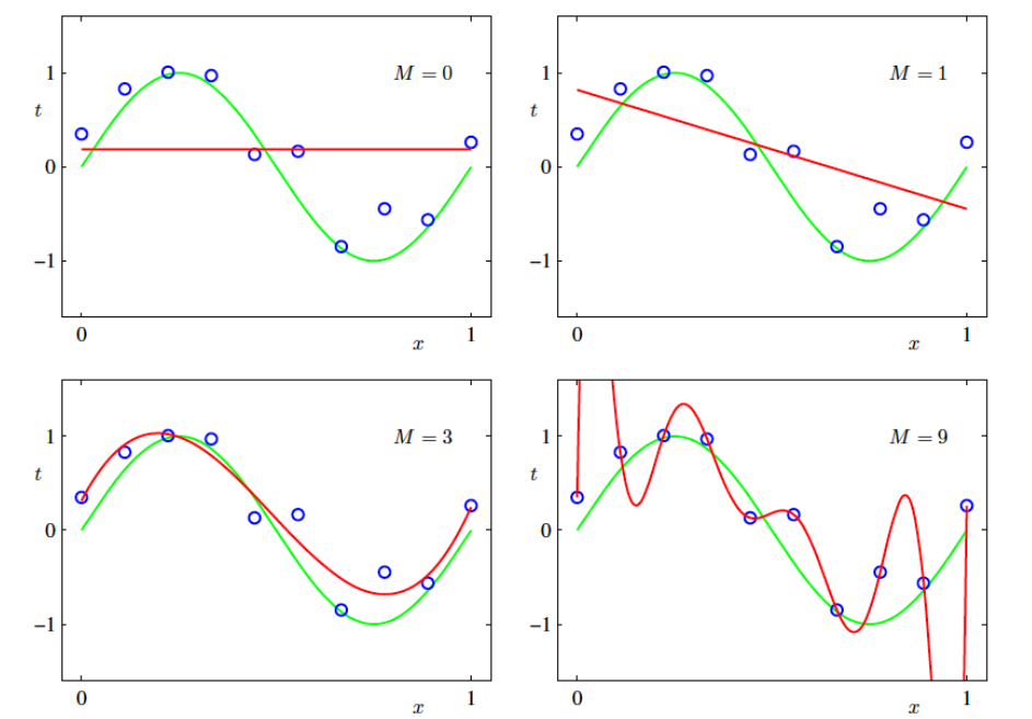
In some cases, even a polynomial function may not pass through all our training data points. While we can increase the polynomial’s degree to make it pass through every point, doing so may lead to poor generalization performance. This phenomenon is known as overfitting, where the model performs well on training data but not on new, unseen data. Therefore, for a reasonably chosen value of M, we need to focus on minimizing the error that the model makes.
Here in the below image, green curve is the actual function. Red is our model. A higher order polynomial (\(M=9\)) provides excellent fit to the training data but bad generalization performance.
The first order polynomial has high train and test error, the 9th-order polynomial has zero train error and very high test error. There exist some polynomial in the middle which could give a good train and test performance. The weight coefficients learned are as below:
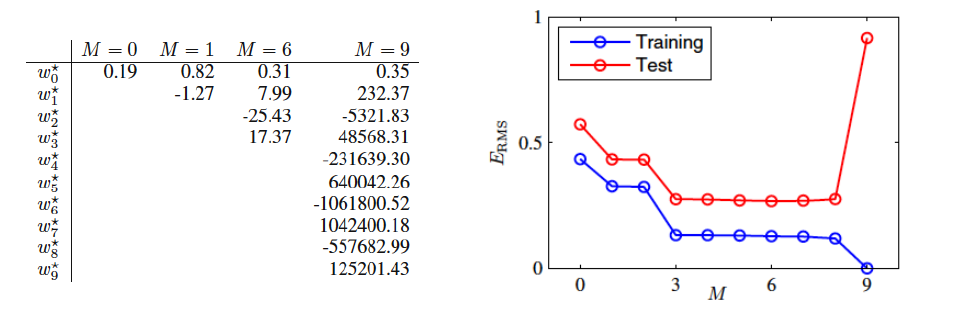
For regression models, performance is calculated using the root square mean error:
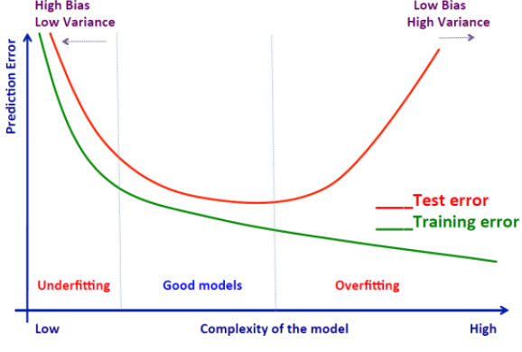
The typical behaviour is:
|
Note
|
Given model complexity, the over-fitting problem become less severe as the data size increases. |
To determine the optimal value of \(M\), split the data into training, validation, and test sets. Train polynomial models of varying orders on the training data and evaluate their performance on the validation set. Select the model that yields the best performance. However, this process can be time-consuming and computationally expensive.
An alternative approach is to allow a higher-order polynomial to learn a simpler function through regularization. Regularization constrains the weight coefficients during training.
For instance, in a 9th-order polynomial, the weight coefficients can become excessively large. To fit all observations, the function fluctuates significantly, leading to unnecessary complexity. This happens because large coefficients force the function to oscillate more. By applying a regularization term, we restrict the growth of these coefficients, resulting in a smoother and more stable function.
Regularization
If we can somehow restrict the weight coefficient values from growing too large, we can learn some smooth function like a third order polynomial using a 9th-order polynomial as well. So we add a penalty term to the error function in order to discourage the coefficients from reaching large values.
|
Note
|
For simplicity, consider all the basis functions as simple functions \(\phi_j(\mathbf{x}_n) = x_{nj}\) for \(j=0, 1, \dots, D\) |
where \(w_1^2 + \dots + w_{M-1}^2 = \lVert \mathbf{\tilde{w}} \rVert^2 = \mathbf{\tilde{w}}^\top \mathbf{\tilde{w}}\). This error is known as regularized least squares error. Here we have used the \(L2\) norm and this version of regression model is known as Ridge regression.
|
Important
|
Notice that the intercept \(w_0\) has been left out of the penalty term. |
We aim to learn \(\mathbf{w}\) such that the combination of squared error and the \(L2\) norm of the coefficient vector is minimized. Regularization helps prevent high-order polynomials from taking excessively large coefficient values.
The regularization constant \(\lambda\) is a hyperparameter that balances the importance of the norm term and the data fit term. It can take any positive value. In Scikit-learn and other packages, the default value of \(\lambda\) is 1.
-
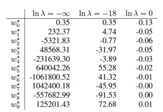
When \(\ln \lambda\) is very small, the regularization term is almost ignored. We end up overfitting.
-
When \(\ln \lambda\) is very large, excessive importance is given to the regularization term. We end up underfitting.
We need to fine tune and come up with the right value of \(\lambda\) using the validation data set. Try values such as 0.01, 0.1, 1, 10, 100, 1000.
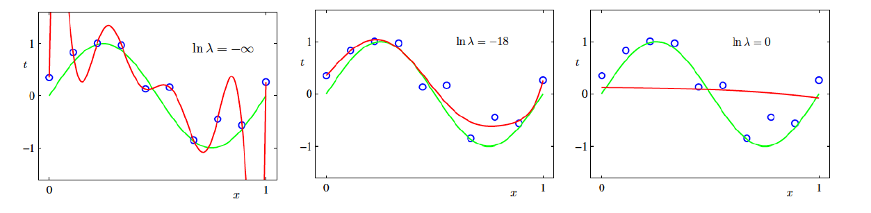
Note: In this case, we have fit a 9th-order polynomial using different values of \(\lambda\). Instead of choosing the appropriate polynomial order, the problem is now reduced to selecting the right hyperparameter value. Hyperparameter tuning is generally preferred as it tends to be less sensitive.
Ridge Regression
Our objective for ridge regression is
The solution to this can be separated into two parts:
-
Setting the derivative with respect to \(w_0\) equal to 0, and solving for \(w_0\), we obtain
\[\hat{w}_0 = \frac{1}{N} \sum_{n=1}^N t_n - \frac{1}{N} \sum_{n=1}^N \sum_{j=1}^D w_j x_{nj}\]As we notice, this involves \(w_j\)'s that we are yet to estimate. We can put the optimal value of \(\hat{w}_0\) in the objective function as below and solve for \(w_j\) for \(j=1, \dots D\).
\[\arg \min_{\mathbf{w}} \left\{ \frac{1}{2} \sum_{n=1}^N \left(t_n - \frac{1}{N} \sum_{n=1}^N t_n - \frac{1}{N} \sum_{n=1}^N \sum_{j=1}^D w_j x_{nj} - \sum_{j=1}^D w_j x_{nj} \right)^2 + \frac{\lambda}{2} \sum_{j=1}^D w_j^2 \right\}\]But this is a cumbersome process. Fortunately when each feature has zero mean, the second term in \(\hat{w}_0\) vanishes:
\[\sum_{n=1}^N \sum_{j=1}^D w_j x_{nj} = \sum_{j=1}^D w_j \left( \sum_{n=1}^N x_{nj} \right) = 0\]Therefore, \(\hat{w}_0 = \frac{1}{N} \sum_{n=1}^N t_n\). It is a constant, it doesn’t involve any \(w_j\), i.e., it is independent of them. As a constant doesn’t affect our solution, the objective function can simply be considered as
\[\arg \min_{\mathbf{w}} \left\{ \frac{1}{2} \sum_{n=1}^N \left(t_n - \sum_{j=1}^D w_j x_{nj} \right)^2 + \frac{\lambda}{2} \sum_{j=1}^D w_j^2 \right\}\] -
The remaining co-efficients can be estimated by a ridge regression without intercept, using the centered \(x_{nj}\). Henceforth on assuming that this centering has been done, so that the input matrix \(\mathbf{X}\) has \(D\) columns (rather than \(D+1\)) columns and \(\mathbf{w}\) also has \(D\) coefficients.
\[\begin{align*} E(\mathbf{w}) & = \frac{1}{2} \sum_{n=1}^N (t_n - y_n )^2 + \frac{\lambda}{2} \lVert \mathbf{w} \rVert^2 \\ & = \frac{1}{2} \left( \mathbf{y} - \mathbf{X w} \right)^\top \left( \mathbf{y} - \mathbf{X w} \right) + \frac{\lambda}{2} (\mathbf{w}^\top\mathbf{w})\\ & = \frac{1}{2} \left( \mathbf{t}^\top \mathbf{t} - 2\mathbf{t}^\top \mathbf{Xw} + \mathbf{w}^\top \mathbf{X}^\top \mathbf{X}\mathbf{w} \right) + \frac{\lambda}{2} (\mathbf{w}^\top \mathbf{w}) \end{align*}\]\[\begin{align*} \nabla E(\mathbf{w}) = \frac{\partial E(\mathbf{w})}{\partial \mathbf{w}} & = \mathbf{0}^\top \\ \frac{1}{2} \left( - 2\mathbf{t}^\top \mathbf{X} + \hat{\mathbf{w}}^\top \mathbf{X}^\top \mathbf{X} + \mathbf{X}^\top \mathbf{X} \hat{\mathbf{w}} + 2\lambda \hat{\mathbf{w}}^\top \right) & = \mathbf{0}^\top \\ - \mathbf{t}^\top \mathbf{X} + \hat{\mathbf{w}}^\top \mathbf{X}^\top \mathbf{X} + \lambda \hat{\mathbf{w}}^\top & = \mathbf{0}^\top \\ \hat{\mathbf{w}}^\top \left( \mathbf{X}^\top \mathbf{X} + \lambda \mathbf{I} \right) & = \mathbf{t}^\top \mathbf{X} \\ \hat{\mathbf{w}}^\top & = \mathbf{t}^\top \mathbf{X} (\mathbf{X}^\top \mathbf{X} + \lambda \mathbf{I} )^{-1} \\ \Rightarrow \hat{\mathbf{w}} & = (\mathbf{X}^\top \mathbf{X} + \lambda \mathbf{I} )^{-1} \mathbf{X}^\top \mathbf{t} \end{align*}\]
This is known as the ridge regression regularized least squares solution. Notice that with the choice of quadratic penalty \(\mathbf{w}^\top\mathbf{w}\), the ridge regression solution is a linear function of \(\mathbf{t}\).
Lasso Regression
The objective for lasso regression is
Notice the similarity to the ridge regression problem: the L2 ridge penalty \(\sum_1^D w_j^2\) is replaced by L1 lasso penalty \(\sum_1^D |w_j|\). This latter constraint makes the solutions nonlinear in \(\mathbf{t}\), and there is no closed form expression as in ridge regression. Computing the lasso solution is a quadratic programming problem.
Ridge Vs Lasso
A commonly used regularization involves adding the square of the \(L2\) norm of the weight coefficients to the objective function. This choice is popular due to its desirable properties, such as continuity and differentiability. However, other norms can also be used.
In general, the \(L_p\) norm of the weight coefficients vector is given by:
On comparing the \(L1\) norm and the \(L2\) norm, we observe that
The \(L1\) norm causes weight coefficients to shrink to zero much faster than the \(L2\) norm.
To see this, note that the error function consists of two components: data loss and regularization loss. Considering only the regularization loss, let’s examine a simple case with a single weight coefficient \(w\). The plot below shows the L1 and L2 norm error for different values of \(w\)
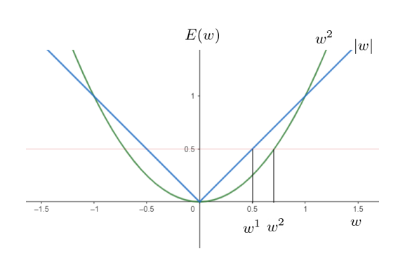
For \(E(w)=0.5\), let \(w^1\) be the corresponding weight coefficient using the L1 norm function and \(w^2\) using the L2 norm function. We observe that \(w^1\) is closer to zero than \(w^2\). This indicates that as the error decreases, the L1 norm drives weight coefficients to zero more quickly than the L2 norm.
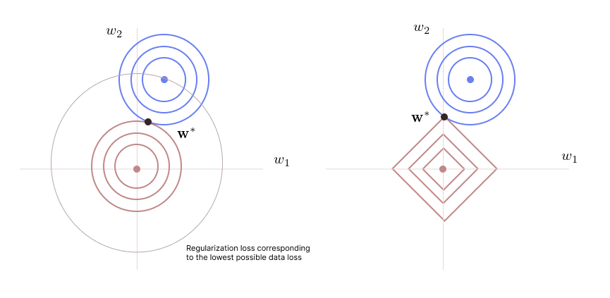
When we have two weight coefficients \(w_1\) and \(w_2\), the plot of the data loss (blue circles) and the regularization loss (red) for different values of the total loss is given by:
-
Left plot: The blue concentric circles represent the data loss. The red concentric circles represent the regularization loss when using the \(L_2\) norm \(w_1^2 + w_2^2 = k\). Each circle represents a set of \(w_1\) and \(w_2\) satisfying this equation for a specified regularization loss \(k\). As we move out of the blue circles, the data loss will be higher. As we move out of the red circles, the regularization loss will be higher. The optimal point \(\boldsymbol{w}^*\) is where both the losses are minimized.
-
Left plot: The blue concentric circles represent the data loss. The diamond-shaped contours represent the regularization loss when using the \(L_1\) norm \(|w_1| + |w_2| = k\). Each contour represents a set of \(w_1\) and \(w_2\) satisfying this equation for a specified regularization loss \(k\). As we move out of the blue circles, the data loss will be higher. As we move out of the diamond-shaped contours, the regularization loss will be higher. The optimal point \(\boldsymbol{w}^*\) is where both the losses are minimized. In this case, the optimal solution often lies on one of the axes, forcing \(w_1\) to zero.
Thus, the L1 norm can be used when we want to retain only important variables while eliminating others.
References
-
Christopher M. Bishop Pattern Recognition and Machine Learning. Springer (2006)
-
Hastie, T., Tibshirani, R., & Friedman, J. (2013). The elements of statistical learning: Data Mining, Inference, and Prediction. Springer Science & Business Media.