How do we find the best-fit line through a cloud of data points? The Least Squares Method holds the key! By minimizing errors, this simple yet powerful technique makes Linear Regression the go-to tool for predictions.
Problem Formulation
Given training data \(\{(\mathbf{x}_n, t_n)\}\) for \(n =1,2,\dots, N\) where \(\mathbf{x}_n \in \mathbb{R}^{D}, t_n \in \mathbb{R}\).
-
\(\mathbf{x}_n\) represents the \(n\)th training case, a vector containing the values \(\{x_{n1}, x_{n2}, x_{n3}, \dots, x_{nD}\}\).
-
\(t_n\) is the true label corresponding to the \(n\)th training case.
Our goal is to learn a function that maps these inputs to outputs \(f: \mathbf{x}_n \rightarrow t_n\).
A simple assumption is that each \(t_n\) can be expressed as the weighted combination of the predictor variables (after proper scaling) plus a bias term \(w_0\). The bias term is added to adjust the output to the range of \(t_n\). For \(N\) observations, this results in a system of linear equations:
A straight-forward approach to finding the coefficients \(w\)'s would be to solve this system of linear equations. However, in practice, an exact solution often does not exist unless all observations lie on a straight line. Observations never lie on a straight line because of measurement errors. Consequently, we must adopt alternative approaches.
Least Squares Estimate
We aim to find a line (or hyperplane) that is as close as possible to all data points. This means learning the coefficients in a way that minimizes the distance between the predicted and actual values.
Consider a linear function (linear in parameters): \(y_n = w_0 x_{n0} + w_1 x_{n1} + \dots + w_D x_{nD} = \mathbf{w}^\top \mathbf{x}_n\), where \(x_{n0}=1\) for all \(n\) and \(y_n\) is the predicted value of our model using some weight vector \(\mathbf{w}\). Our goal is to make these predictions as close as possible to the actual values.
To achieve this, we learn \(\mathbf{w} \in \mathbb{R}^{D+1} \) by minimizing the sum of squared errors between \(t_n\) and \(y_n\). The error \(E\), a function of \(\mathbf{w}\), is known as the squared error. On dividing it by \(N\), we get the mean squared error. But for mathematical convenience, we divide it by 2.
We need \(\mathbf{w}\) such that the function MSE is minimum. This approach of finding the optimal \(\mathbf{w}\) is known as least squares error method.
To optimize this, we can find the gradient of the objective function \(E(\mathbf{w})\) and equate it to 0.
|
Caution
|
In the above derivation, we assume that \(\mathbf{X}^\top \mathbf{X}\) is invertible. |
For linear regression, we have a closed-form expression for finding the optimal \(\mathbf{w}\) as an analytic function of \(\mathbf{X}\) and \(\mathbf{t}\).
Linear Basis Function Models
The simplest linear model for regression is one that involves a linear combination of the input variables (which we saw above)
where \(x_{n0} = 1\). This model is often simply known as a linear regression model. The key property of this model is that it is a linear function of the parameters \(w_0, w_1, \dots, w_D\). It is also, however, a linear function of the input variables \(x_0, x_1, \dots, x_D\), and this imposes significant limitations on the model. We therefore extend the class of models by considering linear combinations of fixed nonlinear functions of the input variables, of the form
where \(\phi_j(\mathbf{x}): \mathbb{R}^D \rightarrow \mathbb{R}\) are known as basis functions. Note that the total parameters of this model is \(M\). In matrix notation, the model can be written as
Where
By using nonlinear basis functions, we allow the function \(y(\mathbf{x}, \mathbf{w})\) to be a nonlinear function of the input vector \(\mathbf{x}\). But still functions of the above form are called linear models, because this function is linear in parameters \(\mathbf{w}\).
Example: Polynomial Regression
Say we are given a dataset with a single feature and a target \(\{(x_n, t_n)\}\) for \(n =1,2,\dots, N\), where \(x_n, t_n \in \mathbb{R}\). And we see that \(t\) and \(\mathbf{x}\) are related in a non-linear manner. If we assume that the function is a \(M\)th order polynomial, then we can write the function involving one variable as:
Here the basis functions are \(\phi_0(x) = 1, \, \phi_1(x) = x, \, \phi_2(x) = x^2, \, \phi_M(x) = x^M\). Here we map an input \(x \in \mathbb{R}\) to a (M+1)-dimensional space \(\mathbb{R}^{M+1}\). On considering all the training data cases \(n=1\) to \(N\), we can write the design matrix \(\boldsymbol{\Phi}\) as:
The squared error is:
Then our optimal \(\mathbf{w}\) is
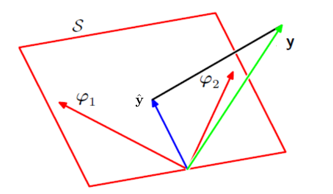
Geometric Interpretation of Least Squares
In general, we have \(M\) features (number of columns), each of which can be represented through basis functions \(\phi_j(\mathbf{x})\).
Given these features, we are doing a linear combination of these features to get out output \(\mathbf{t}\).
We cannot find a \(\mathbf{w}\) that satisfies all these \(N\) equations, so we find the coefficients in such a way that it minimizes the difference between \(\boldsymbol{\Phi} \mathbf{w}\) and \(\mathbf{t}\). And we end up learning our coefficients as:
On substituting the value in the previous equation, we get:
We have actually applied a matrix transformation \(\boldsymbol{\Phi} (\boldsymbol{\Phi}^\top \boldsymbol{\Phi})^{-1} \boldsymbol{\Phi}^\top\) to \(\mathbf{t}\) to get our predicted output.
The least squares regression function is obtained by finding the orthogonal projection of the N-dimensional output vector \(\mathbf{t}\) onto the subspace spanned by the basis functions \(\phi_j(\mathbf{x})\) vectors that are N-dimensional vectors. Since there are only \(M\) vectors and typically \(M < N\), it cannot span the whole space, it spans only a subspace.
References
-
Christopher M. Bishop Pattern Recognition and Machine Learning. Springer (2006)
-
Kevin P. Murphy Machine Learning: a Probabilistic Perspective, the MIT Press (2012), also see upcoming 2021 editions https://probml.github.io/pml-book/