In single-variable calculus, the derivative tells us how a function changes at a point - how steep the hill is under your feet. But as we step into higher dimensions, the concept evolves dramatically. Suddenly, we’re not just talking about slopes, but about gradients that point in the direction of greatest change, Jacobians that capture how systems distort space.
Review of Linear Maps
The idea of linear maps helps us understand the (first-order) derivatives much better, especially in high dimensional spaces. So, a quick recap of this is as follows.
We know that a vector-valued linear function \(f: \mathbb{R}^n \to \mathbb{R}^m\) can be represented by \(f(\mathbf{x}) = \mathbf{Ax}\), where \(\mathbf{A}\) is an \(m \times n\) matrix. In linear algebra, we look at this as a linear mapping from the vector space \(\mathbb{R}^n\) to the vector space \(\mathbb{R}^m\). When we fix the standard basis for \(\mathbb{R}^n\) and \(\mathbb{R}^m\), every linear map \(f: \mathbb{R}^n \to \mathbb{R}^m\) corresponds to a unique matrix \(\mathbf{A} \in \mathbb{R}^{m \times n}\) such that
That is, once the basis is fixed, the matrix fully determines the linear map. So, with a bit of abuse of language, it is common to say "Let \(\mathbf{A} \in \mathbb{R}^{m \times n}\) be a linear map". But what it really means is: "Let \(f(\mathbf{x}) = \mathbf{Ax}\) be a linear map".
Derivative of Single Variable Functions
Let \(f: \mathbb{R} \to \mathbb{R}\). For \(h>0\), the derivative of \(f\) with respect to \(x\) at \(x_0\), denoted by \(f'(x_0)\) or \(\frac{d f}{d x}(x_0)\), is defined as
provided the limit exists. The function \(f\) is differentiable at \(x_0\) iff this limit exists. And this limit value is itself called as the derivative of the function at \(x_0\). This measures the instantaneous rate at which the function \(f\) changes for a inifinitesimal small change from \(x_0\). \(f(x)\) is called differentiable on an interval if the derivative exists for every point in that interval.
Alternate Definition:
Let \(f: \mathbb{R} \to \mathbb{R}\) be any function. We can approximate this function at a point \(x_0\) using a linear function. Such a linear function should
-
Exactly equal \(f(x_0)\) at \(x_0\).
-
The error we make by approximating the original function by this linear function should decay to 0 as we move towards \(x_0\). The error should decay to 0 at least as fast as the distance \(|x-x_0|\) decay to 0. That is, the error should at least be quadratic to the distance \(|x-x_0|\), i.e., it should be \(|x-x_0|^2\). In general, the linear approximation error should be quadratic, the quadratic approximation error should be cubic, etc.
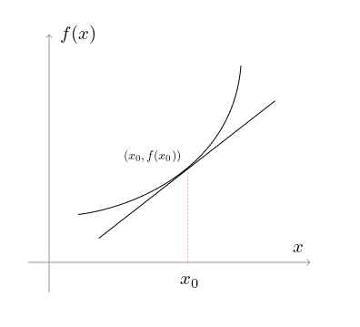
Say we are at \(x_0\), the function value is \(f(x_0)\). A line passing the point \((x_0, f(x_0))\) can be written as \(f(x) - f(x_0) = m(x-x_0)\).
The linear (affine) function
is called the first-order approximation of \(f\) at (or near) \(x_0\). The error in approximating the original function by this linear function is given by \(f(x) - (f(x_0) + m(x-x_0))\). If there exists an \(m\) such that
goes to 0, then we say the function is differentiable at \(x_0\). And we call this \(m\) as the derivative of \(f\) at \(x_0\). Then we can write
For example, let the function be \(f(x)=x^2\) with \((x_0,f(x_0)) = (3,9)\) and we know that \(f'(x_0) = 6\).
This is the linear approximation of \(x^2\) at \(x=3\). We can see that, as we get closer to 3, the RHS gets closer to 9. On writing it as:
So, to know the change in \(f\), we can just multiply the change in \(x\) by \(f'(x_0)\). This becomes:
as we take the infinitesimal limit (as the change in \(x\) tends to 0). Comparing this form with Equation 1 helps us see that "the derivative of a function at a point is the unique linear map that best approximates the change in the function’s value near that point".
The derivative at \(x_0\) is commonly interpreted (especially in high school calculus) as the slope of the tangent line at \(x_0\), or as the instantaneous rate of change of the function at \(x_0\)
However, a more rigorous and modern view defines the derivative as a linear map.
The derivative at \(x_0\), viewed as a linear map, takes a small input increment \(dx \in \mathbb{R}\) and maps it to \(f'(x_0) \cdot dx\), which is the best linear approximation to the change in the function value \(f(x_0+dx) - f(x_0)\).
So, to find the derivative of \(f\) at \(x_0\), instead of solving Equation 2, we can derive the first-order approximation of \(f\) at \(x_0\) and find an \(m\) that satisfies Equation 3.
Derivative of Multivariable Functions
Let \(f: \mathbb{R}^n \rightarrow \mathbb{R}\) be a multivariable scalar-valued function. Similar to the single-variable case, the derivative of a multivariable function is fundamentally about measuring the rate at which the function changes. However, with multiple independent variables, the notion of the "rate of change" becomes more nuanced as we can consider changes with respect to each variable or along any specific direction among the countably infinite directions.
Thus, there are different forms of derivatives.
Partial Derivatives
The partial derivatives measure the rate of change of a multivariable function with respect to one variable, while holding all other variables constant. For a function \(f(x_1, x_2)\), keeping \(x_2\) fixed, we may want to know how \(f\) changes as \(x_1\) changes: \(\frac{\partial f}{\partial x_1}\). This is defined as
Directional Derivatives
The directional derivatives generalize the partial derivative to measure the rate of change of a function along an arbitrary direction (given by a unit vector \(\mathbf{u}\)). Say we are at \(\mathbf{x}_0 \in \mathbb{R}^n\) and we are given a direction \(\mathbf{u} \in \mathbb{R}^n\). On restricting the movement along the \(\mathbf{u}\) direction, we end up with this restricted function \(f(\mathbf{x}_0 + h \mathbf{u})\) where \(h\) is a scalar, and this is a function of a single variable \(h\).
We can find the derivative of this single variable function, \(g'(h)\). This \(g'(h)\) is called as the directional derivative of \(f\) at \(x_0\) in the direction \(\mathbf{u}\). We get one directional derivative for every direction \(\mathbf{u}\).
Formally, the instantaneous rate of change of \(f(\mathbf{x})\) at \(\mathbf{x}_0\) in the direction \(\mathbf{u}\) is called the directional derivative and is denoted by \(D_{\mathbf{u}} f(\mathbf{x}_0)\)
The directional derivative in the standard directions of the vector space gives us the partial derivatives. We know that in a vector space, we can express any vector as a linear combination of the basis vectors. These basis vectors form the standard directions. For example, for the function \(f: \mathbb{R}^2 \rightarrow \mathbb{R}\), the standard directions are \(\mathbf{u} = (1,0)\) and \((0,1)\). Then
Derivatives of these single variable functions are the partial derivatives of \(f\) at \(\mathbf{x_0}\). Suppose \(f(\mathbf{x}) = x_1^2 + x_2^2\), then
The derivative of these functions give us \(\frac{\partial f}{\partial x_1}\) and \(\frac{\partial f}{\partial x_2}\) at \((x_1,x_2)\). And we know that,
Gradient
The gradient of a scalar-valued multivariable function at a point \(\mathbf{x}_0\), often denoted by \(\nabla f(\mathbf{x}_0)\), is a vector whose components are the partial derivatives of the function at \(\mathbf{x}_0\). For \(f(x_1, x_2)\), the gradient at \((x_1, x_2)\) is
The gradient is always a column vector and this vector points in the direction of the greatest rate of increase of the function. For every scalar-valued multivariable function, the gradient will always have the same shape as the input. So, it will be in the same space as the input vector.
Total Derivative
Let \(f: \mathbb{R}^n \rightarrow \mathbb{R}\). How can we define the differentiability of the function at a point \(\mathbf{x_0}\)? We can follow the same method that we did for the single variable case. The linear (affine) function
is called the first-order approximation of \(f\) at (or near) \(\mathbf{x}_0\). The error in approximating the original function by this linear function is given by \(f(\mathbf{x}) - (f(\mathbf{x}_0) + \mathbf{w}^\top (\mathbf{x}-\mathbf{x}_0))\). If there exists a \(\mathbf{w} \in \mathbb{R}^n\) such that
goes to 0, then we say the function is differentiable at \(\mathbf{x}_0\). And we call such \(\mathbf{w}^\top\) as the (total) derivative of \(f\) at \(\mathbf{x}_0\), often denoted by \(D f(\mathbf{x}_0)\). There can be at most one \(\mathbf{w}\) that satisfies this.
Theorem:
If \(f\) is differentiable at \(\mathbf{x}_0\), then the directional derivative \(D_{\mathbf{u}} f(\mathbf{x}_0) = \langle \mathbf{w}, \mathbf{u} \rangle\)
This theorem helps us find \(\mathbf{w}\). When \(\mathbf{u}=(1,0)\), the LHS gives the first partial derivative and the RHS gives the first entry of \(\mathbf{w}\). So, the first entry of \(\mathbf{w}\) should be the first partial derivative, the second entry should be the second partial derivative, etc. \(\mathbf{w}\) should be the gradient of \(f\) at \(\mathbf{x}_0\). Hence, the derivative of \(f\) at \(\mathbf{x}_0\) is
Then we can write
So, to know the change in \(f\), we can just take the dot product of the \(\Delta \mathbf{x}\) vector with the vector \(\nabla f(\mathbf{x}_0)^\top\). This becomes:
as we take the infinitesimal limit (as the change in \(\mathbf{x}\) tends to 0). Comparing this form with Equation 1 helps us see that "the derivative of \(f\) at the point \(\mathbf{x}_0\), \(\nabla f(\mathbf{x}_0)^\top\), is a linear map that best approximates the change in \(f\) near \(\mathbf{x}_0\)." This linear form tells us the first-order approximation of how the function changes in response to a small change in \(\mathbf{x}\).
For scalar-valued multivariable functions, the derivative \(D f(\mathbf{x}_0)\) is a row vector \(\nabla f(\mathbf{x}_0)^\top \in \mathbb{R}^{1 \times n}\), which is the transpose of the gradient vector.
The derivative of a multivariable scalar function \(f\) at \(\mathbf{x}_0\) can be found by the following two ways:
-
From the partial derivatives \(\frac{\partial f}{\partial x_1}, \dots, \frac{\partial f}{\partial x_n}\): this is a tedious task as \(n\) becomes large.
-
By deriving the first-order approximation of \(f\) at \(\mathbf{x}_0\), i.e., the vector \(D f(\mathbf{x}_0)\) that satisfies Equation 4.
Derivative of Vector-Valued Functions
Let \(f: \mathbb{R}^n \rightarrow \mathbb{R}^m\) be a vector-valued function. The function \(f\) is differentiable at \(\mathbf{x}_0\) if there exists a matrix \(Df(\mathbf{x}_0) \in \mathbb{R}^{m \times n}\) that satisfies
in which case we refer to \(Df(\mathbf{x}_0)\) as the derivative (or Jacobian) of \(f\) at \(\mathbf{x}_0\). There can be at most one matrix that satisfies this. The linear (affine) function
is called the first-order approximation of \(f\) at (or near) \(\mathbf{x}_0\). Then
So, to know the change in \(f\), we can just do matrix-vector multiplication of \(\Delta \mathbf{x}\) and \(D f(\mathbf{x}_0)\). This becomes:
as we take the infinitesimal limit (as the change in \(\mathbf{x}\) tends to 0). Comparing this form with Equation 1 helps us see that "the derivative of \(f\) at the point \(\mathbf{x}_0\), \(D f(\mathbf{x}_0)\), is a linear map that best approximates the change in \(f\) near \(\mathbf{x}_0\)."
For vector-valued functions, the derivative \(D f(\mathbf{x}_0)\) is a matrix \(\mathbb{R}^{m \times n}\), which is known as the Jacobian.
The derivative of a vector-valued function \(f\) at \(\mathbf{x}_0\) can be found by the following two ways:
-
From the partial derivatives \(Df(\mathbf{x}_0)_{ij} = \frac{\partial f_i}{\partial x_j}, \,\, \, i=1, \dots, m, \,\, j=1,\dots,n\): this is obviously a tedious task.
-
By deriving the first-order approximation of \(f\) at \(\mathbf{x}_0\), i.e., the matrix \(D f(\mathbf{x}_0)\) that satisfies Equation 5.
Summary
Depending upon the nature of input and output of the function, the derivative takes appropriate forms. The following table summarizes the derivative structure for functions whose input and output are:
| Input \(\downarrow\) / Output \(\to\) | Scalar | Vector | Matrix |
|---|---|---|---|
Scalar |
Scalar |
Vector |
Matrix |
Vector |
Row vector (transpose of the gradient vector) |
Matrix (Jacobian matrix) |
Higher order array |
Matrix |
Matrix |
Higher order array |
Higher order array |
These represent the explicit notation of the derivative for different cases. An implicit view is to look at the derivative as a "linear operator" \(D f(\mathbf{X})\) acting on perturbation \(d\mathbf{X}\).
|
Note
|
Scalars are zero dimensional, vectors are 1 dimensional, matrices are two dimensional arrays, etc. The size(scalar) is [], size(vector) is \([n]\), size of a matrix is \([m,n]\), etc. |
References
-
Boyd, S. P., & Vandenberghe, L. (2004). Convex Optimization. Cambridge University Press.
-
MIT OpenCourseWare. (n.d.). MIT OpenCourseWare. https://ocw.mit.edu/courses/18-s096-matrix-calculus-for-machine-learning-and-beyond-january-iap-2023/resources/ocw_18s096_lecture01_part1_2023jan18_mp4/
-
S2.2. (n.d.). https://www.math.toronto.edu/courses/mat237y1/20189/notes/Chapter2/S2.2.html
-
14.5 directional derivatives. (n.d.). https://www.whitman.edu/mathematics/calculus_online/section14.05.html