A formal definition of functions. And when do we call a function linear, affine, or quadratic?
What are Functions?
A function is defined between two sets, \(A\) and \(B\). It is just a mapping with some unique properties. We write \(f: A \rightarrow B\) to mean that \(f\) is a function on the set \(\mathcal{D} \subseteq A\) into the set \(\mathcal{R} \subseteq B\). The set \(\mathcal{D}\) is the domain, the set \(B\) is the codomain, and the set \(\mathcal{R}\) is the range of the function.
-
Domain: The set \(\mathcal{D}\) contains all inputs \(\mathbf{x}\) for which the function is defined. In particular, we can have \(\mathcal{D}\) a proper subset of the set \(A\).
-
Codomain: The set \(B\) contains all potential outputs of the function, even if some elements of \(B\) are never actually attained by \(f\).
-
Range: The set \(\mathcal{R}\) contains the actual outputs attained by \(f\).
Thus, the notation \(f: \mathbb{R}^n \to \mathbb{R}\) means that \(f\) maps (some) \(n-\) vectors into (some) \(\mathbb{R}\); it does not mean that \(f(\mathbf{x})\) is defined for every \(\mathbf{x} \in \mathbb{R}^n\), and the \(f\) outputs all scalar in \(\mathbb{R}\).
Scalar-valued functions:
Let \(\mathcal{D} \subseteq \mathbb{R}^n\). A real valued scalar function \(f: \mathbb{R}^n \to \mathbb{R}\) on \(\mathcal{D}\) is a rule that assigns a real number
for all element in \(\mathcal{D}\). Here \(\mathbf{x} = (x_1, \dots, x_n)\) are independent variables and \(y\) is a dependent variable.
Vector-valued functions:
A function \(f\) that carries every element of \(\mathcal{D}\) to some element in \(\mathbb{R}^m\), \(f: \mathbb{R}^n \to \mathbb{R}^m\), that is, the function takes a \(n-\) vector and outputs an \(m-\) vector.
-
The domain of \(f\) is \(\mathcal{D}\) which is a set of all points \(\mathbf{x}\) in \(\mathbb{R}^n\) for which \(f(\mathbf{x})\) is defined.
-
The range of \(f\) is \(\mathcal{R}\) which is a set of all points \(y\) in \(\mathbb{R}\) (in case of scalar-valued functions) or \(\mathbf{y}\) in \(\mathbb{R}^m\) (in case of vector-valued functions) such that \(\mathbf{y}=f(\mathbf{x})\) for all \(\mathbf{x} \in \mathcal{D}\).
Properties of Functions
Let \(f: \mathbb{R}^n \to \mathbb{R}\)
-
The graph of \(f\) is defined as
-
The epi-graph of \(f\) is the set of all points including the graph and above the function.
\[epi(f) \equiv \{(x_1, \dots, x_n,y) \,|\, \mathbf{x} \in \mathcal{D}, y \geq f(\mathbf{x})\}\] -
The level-set (contour) of \(f\) at some level \(\alpha\) is the set of points in the domain of the function where the function takes on a constant value \(\alpha\)
\[\mathcal{L}_f(\alpha) \equiv \{\mathbf{x} \in \mathcal{D} \,|\, f(\mathbf{x}) = \alpha\}\]
Example 1:
Consider the function \(f(x_1, x_2) = x_1^2 + x_2^2\). Cut the \(f(\mathbf{x})\) axis at \(\alpha=1\). And look for the points that achieve \(f(\mathbf{x}) = \alpha\), that is, \(x_1^2 + x_2^2=1\) to get the level set corresponding to value \(\alpha\). It is a subset of the domain.
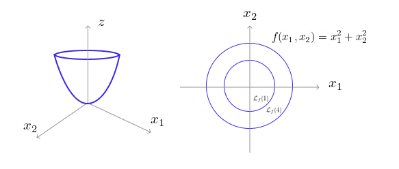
\(\mathcal{L}_f(4)\) is the set of all points on the boundary of the circle of radius 2. As we increase \(\alpha\), we get concentric circles.
Example 2:
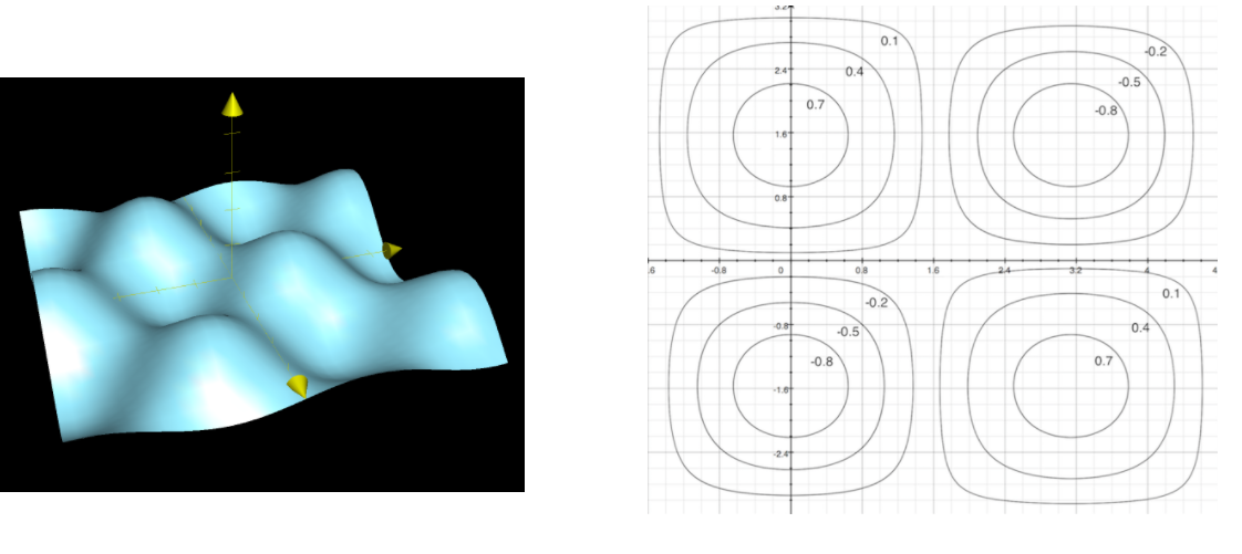
Consider the function \(f(x_1, x_2) = \cos x_1 \cdot \sin x_2\).
|
Caution
|
Peaks and valleys can easily look very similar on a contour plot, and can only be distinguished by reading the labels. |
Example 3:
Consider a linear function \(f(x_1, x_2) = x_1 + 2x_2\)
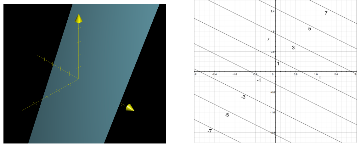
For functions of two variables, contour plots make it much easier to understand the "shape" of the function. From a contour plot
-
We can tell how steep a portion of the graph is by how close the contour curves are to one another. When they are far apart, it takes a lot of lateral distance to increase the function value, but when they are close, the function value increases quickly for small lateral increments.
-
The level sets associated with heights that approach a peak of the graph will look like smaller and smaller closed loops, each one encompassing the next. We can spot the maximum or minimum of a function using its contour plot.
Linear Functions
A function \(f: \mathbb{R}^n \to \mathbb{R}\) is said to be linear if it satifies
-
\(f(\mathbf{x}_1 + \mathbf{x}_2)= f(\mathbf{x}_1) + f(\mathbf{x}_2)\) for any \(\mathbf{x}_1, \mathbf{x}_2\) in the domain of the function.
-
For any \(\alpha \in \mathbb{R}\), \(f(\alpha \mathbf{x}) = \alpha f(\mathbf{x})\).
Example 01:
Consider the function \(f(\mathbf{x}) = w_1x_1 + w_2x_2 + \dots + w_n x_n = \mathbf{w}^\top \mathbf{x}\) where \(x_1, \dots, x_n\) are the elements of the vector \(\mathbf{x}\) and \(w_i \in \mathbb{R}\) for \(i=1,\dots,n\) are the elements of the vector \(\mathbf{w}\). Note here that \(\mathbf{w}\) is a constant and \(\mathbf{x}\) is a variable. Prove that \(f\) is a linear function in terms of \(\mathbf{x}\).
The domain of this function is \(\mathbb{R}^n\). Let \(\mathbf{x}_1 = (x_{11}, \dots, x_{1n}), \mathbf{x}_2 = (x_{21}, \dots, x_{2n}) \in \mathbb{R}^n\). Then, \(\mathbf{x}_1 + \mathbf{x}_2 = (x_{11} + x_{21}, \dots, x_{1n} + x_{2n}) \in \mathbb{R}^n\).
This function satisfies both the conditions, hence it is a linear function in \(\mathbf{x}\).
-
When \(n=1\), then the function is \(f(x) = w_1x\), which is a straight line passing through the origin.
-
when \(n=2\), then the function is \(f(\mathbf{x}) = w_1x_1 + w_2x_2\), which is a plane passing through the origin.
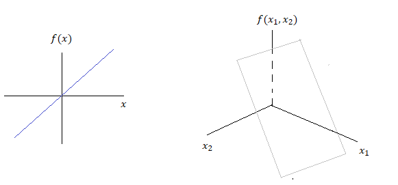 Figure 4. Linear functions \(f(x) = w_1x\) (left) and \(f(\mathbf{x}) = w_1x_1 + w_2x_2\) (right).
 -
When \(n=3\), then the function is \(f(\mathbf{x}) = w_1x_1 + w_2x_2 + w_3x_3\). We can’t visualize this graph as it should be in 4D.
The definition of linear functions can be extended to vector-valued functions \(f: \mathbb{R}^n \to \mathbb{R}^m\), where each component \(f_i(\mathbf{x})\) is a scalar linear function. The function takes a vector \(\mathbf{x} \in \mathbb{R}^n\) and outputs a vector \(\mathbf{y} \in \mathbb{R}^m\).
This function also satisfies both the conditions and thus it is a linear function in \(\mathbf{x}\).
|
Warning
|
A linear function has no intercept, it passes through the origin. |
Affine Functions
We say a function \(g: \mathbb{R}^n \rightarrow \mathbb{R}^m\) is affine if there is a linear function \(f: \mathbb{R}^n \rightarrow \mathbb{R}^m\) and a vector \(\mathbf{b} \in \mathbb{R}^m\) such that \(g(\mathbf{x}) = f(\mathbf{x}) + \mathbf{b}\) for all \(\mathbf{x} \in \mathbb{R}^n\). An affine function is just a linear function plus an intercept.
For example
-
Scalar-valued function: \(g(\mathbf{x}) = w_1x_1 + w_2x_2 + \dots + w_n x_n + b = \mathbf{w}^\top \mathbf{x} + b\), where \(b \in \mathbb{R}\).
-
Vector-valued function: \(g(\mathbf{x}) = \mathbf{Ax} + \mathbf{b}\), where \(b \in \mathbb{R}^m\).
Quadratic Functions
A quadratic function is a polynomial function of degree 2. A scalar-valued function \(f: \mathbb{R}^n \rightarrow \mathbb{R}\) is said to be a quadratic function when it is of the form
where
-
\(\mathbf{Q} \in \mathbb{R}^{n \times n}\) is a symmetric matrix.
-
\(\mathbf{b} \in \mathbb{R}^n\) is a vector of coefficients.
-
\(c \in \mathbb{R}\) is a scalar.
This form generalizes the univariate quadratic \(\frac{1}{2} ax^2 + bx + c\). This can be extended to vector-valued functions \(f: \mathbb{R}^n \to \mathbb{R}^m\), where each component \(f_i(\mathbf{x})\) is a scalar quadratic function.
where for \(i=1, \dots, m\)
-
\(\mathbf{Q}_i \in \mathbb{R}^{n \times n}\) are symmetric matrices.
-
\(\mathbf{b}_i \in \mathbb{R}^n\) are vector of coefficients.
-
\(c_i \in \mathbb{R}\) are scalars.
|
Note
|
The factor \(\frac{1}{2}\) in the quadratic form is a convention that simplifies gradient and Hessian expressions. It is not required for the definition of quadratic function, but a matter of convention for cleaner derivatives. |
References
-
[KhanAcademy] Images are taken from Khan Academy. (n.d.). https://www.khanacademy.org/math/multivariable-calculus/thinking-about-multivariable-function/ways-to-represent-multivariable-functions/a/contour-maps