Why is the defeat of a Go champion by an AI from DeepMind considered a breakthrough in artificial intelligence, while chess is not seen in the same light?
Motivation
The game of Go is primarily played with human intuition rather than calculating all possible moves to determine the best one. While machines can easily evaluate every potential move and select the optimal choice in a given situation, they struggle to replicate the intuitive understanding that humans naturally possess. Therefore, when an AI, such as the one developed by DeepMind, defeats a Go champion, it is regarded as a significant breakthrough in artificial intelligence.
While a trained model can make predictions based on the functions or rules it has learned, do we truly understand how certain or uncertain the model is about its predictions? In contrast, humans make predictions while considering a degree of belief that is informed by intuition and often reflect some level of uncertainty. This raises the question: how can we incorporate human intuition into our models?
We need our models to realize when they are confident about their predictions and when they are not, i.e., they should exhibit uncertainties. Models should be able to identify the out-of-distribution data and they should not make wrong predictions with high confidence. We can incorporate these uncertainty modelling abilities into our models through Bayesian modelling.
Concept Learning
We will consider a very simple example of concept learning called the number game, based on part of Josh Tenenbaum’s PhD thesis.
The game proceeds as follows. I choose some simple arithmetical concept \(C\), such as prime number, even number, power of 2, etc. I then give you a series of randomly chosen positive examples \(\mathcal{D}= \{x_1, \dots, x_N\}\) drawn from \(C\), and ask you whether some new test case \(\tilde{x}\) belongs to \(C\).
Suppose, for simplicity, that all numbers are integers between 1 and 100. Now suppose I tell you "16" is a positive example of the concept. What other numbers do you think are positive? 17? 6? 32? 99?
It’s hard to tell with only one example, so your predictions will be quite vague. Presumably numbers that are similar in some sense to 16 are more likely. But similar in what way? 17 is similar, because it is "close by", 6 is similar because it has a digit in common, 32 is similar because it is also even and a power of 2, but 99 does not seem similar. Thus some numbers are more likely than others.
We can represent this as a probability distribution, \(p(\tilde{x} \, | \, \mathcal{D})\), which is the probability that \(\tilde{x} \in C\) given the data \(\mathcal{D}\) for any \(\tilde{x} \in \{1,2,\dots, 100\}\). This is called the posterior predictive distribution. To update this posterior predictive distribution based on the observed data, we should first get our updated belief over the possible hypotheses.
Bayesian Approach
Say we are given a data \(\mathcal{D}=\{16, 8, 2, 64\}\). Predict the hypothesis from which these numbers are drawn, i.e., what is the probability that these numbers are drawn from hypothesis \(\theta\)? We start with a probability distribution over a set of hypothesis (a prior distribution), and keep updating this distribution based on every observation (data) that we receive.
-
Start with a prior distribution over the hypotheses, i.e., before observing any data. We probably give very low probability to most of the unnatural hypotheses. The prior distribution over hypotheses is \(p(\theta)\).
-
Obtain the likelihood of observing the given data under a hypothesis. It measures how likely it is to observe the data under a particular hypothesis. It is viewed as a function of hypothesis. \(\mathcal{L}(\theta; \mathcal{D}) = p(\mathcal{D} | \theta)\) is the likelihood of the data given the hypothesis.
-
Hypothesis H1: These numbers are from a set of even numbers from 1 to 100. The set of even numbers is \(\{2,4,\dots, 100\}\), there are 50 elements. Given this hypothesis, the probability of seeing these numbers is \((\frac{1}{50})^4\).
-
Hypothesis H2: These numbers are from a set of powers of 2 from 1 to 100. The set of numbers is \(\{1,2,4,8,16,32,64\}\). Given this hypothesis, the probability of seeing these numbers is \((\frac{1}{7})^4\).
The probability of seeing these observations given hypothesis H2 is higher than the probability of seeing these observations given hypothesis H1.
\[P(D| H2) > P(D| H1)\]If we assume that these numbers are from a set of powers of 2 except 32, the probability of seeing these numbers is even higher \((\frac{1}{6})^4\). But this is a unnatural hypothesis (H3), which no one generally thinks of.
Some complex hypotheses end up getting very high likelihood compared to simple hypotheses. So this likelihood alone is not sufficient to infer the underlying true concept. We want to have a mechanism through which we can introduce the domain knowledge that humans possess, i.e., giving more weightage to H2 than H3. Bayesian modelling helps us bring that domain knowledge along with the data to solve a problem.
-
-
Obtain the posterior distribution by multiplying the prior and likelihood (and by normalizing it). The posterior distribution over the hypothesis given the data is \(p(\theta | \mathcal{D})\). The Bayes' Theorem allows us to do this
\[p(\theta | \mathcal{D}) = \frac{p(\mathcal{D} | \theta) \, p(\theta)}{p(\mathcal{D})}\]This theorem provides us with a way to incorporate our intuition about hypotheses into the problem using the prior \(p(\theta)\). Then, we can obtain the likelihood \(p(\mathcal{D} | \theta)\) of the given data for each of our hypothesis. Then by multiplying the prior \(p(\theta)\) and the likelihood \(p(\mathcal{D} | \theta)\), we can update our beliefs about the hypotheses to obtain the posterior \(p(\theta | \mathcal{D})\).
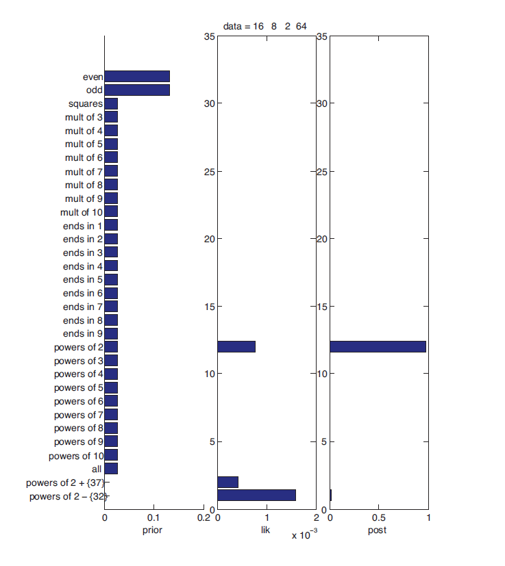
The prior and posterior are probability distributions. They sum (or integrate) to 1. But the likelihood (the plot in the center) is not a probability distribution.
-
Once we have the posterior, we can get the posterior predictive distribution, \(p(\tilde{x} \, | \, \mathcal{D})\).
WarningThe prior, the likelihood and the posterior are over the parameters/hypotheses. But posterior predictive distribution \(p(\tilde{x} \, | \, \mathcal{D})\) is over the (future) data points. The posterior predictive distribution might be
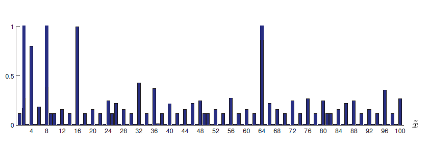
This gives the probability for each \(\tilde{x}\) belonging to the true concept \(C\).
Advantages
What does the Bayesian modelling approach help us do? It mainly allows us to
-
Incorporate domain knowledge: through prior.
-
Model uncertainty: through predictive variance.
-
Generalize from small data: Bayesian model averaging prevents overfitting.
-
Bayesian Optimization: Select the right model from full data: through the evidence or marginal likelihood. In some of the optimization problems, it is costly to compute the objective function and we cannot write it as a function of parameters. One such area is hyperparameter tuning where we find the right model by tuning the hyparameter values. Bayesian optimization helps us find the optimal value of the hyperparameters without trying out a lot of trials.
-
Sequential/Online learning: by considering posterior as prior and training the model on a new dataset to get a new posterior.
-
Active Learning: In a supervised learning setup, it allows us to choose a subset of data that provides the most useful information to the model to learn the underlying function, instead of training the model on all the data points. This is called active learning where we actively select the data points to train the model instead of randomly providing the data. We sample more training data points from a region where the model is uncertain about its prediction. To do this, we should know where the model is uncertain and it should exhibit uncertainty modelling abilities.
The advantages are mentioned at a very high level. No worries if you don’t get it at the moment. As we progress through the series of articles, we will explore each of these concepts in greater detail.
References
-
Murphy, K. P. (2012). Machine learning: A Probabilistic Perspective. MIT Press.