Can a simple algorithm mimic how we think and make decisions? Enter the Perceptron - a groundbreaking idea that transformed AI. But how does this single-layer model draw the line between decisions?
What is a Perceptron?
In 1957, Frank Rosenblatt introduced a more generalized model. This model performs linear classification, but unlike its predecessors, it allows input values to range continuously from \(-\infty\) to \(\infty\). Additionally, it assigns different weights to different input components, providing a mechanism to emphasize certain inputs more than others. Furthermore, it incorporates a learning mechanism for adjusting these weights.
The model outputs 1 when the weighted sum of the inputs exceeds a certain threshold. The outputs are binary.
Here \(\mathbf{w}, b\) are the parameters to be learned. Consider a step function \(\sigma(x)\), which behaves as follows:
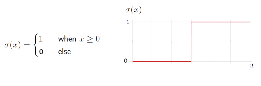
Using this step function, our function \(f(\mathbf{x})\) can be compactly written as
In general, \(\sigma(.)\) is referred to as the activation function. Here, we have used a step function. A single Perceptron can be described as follows:
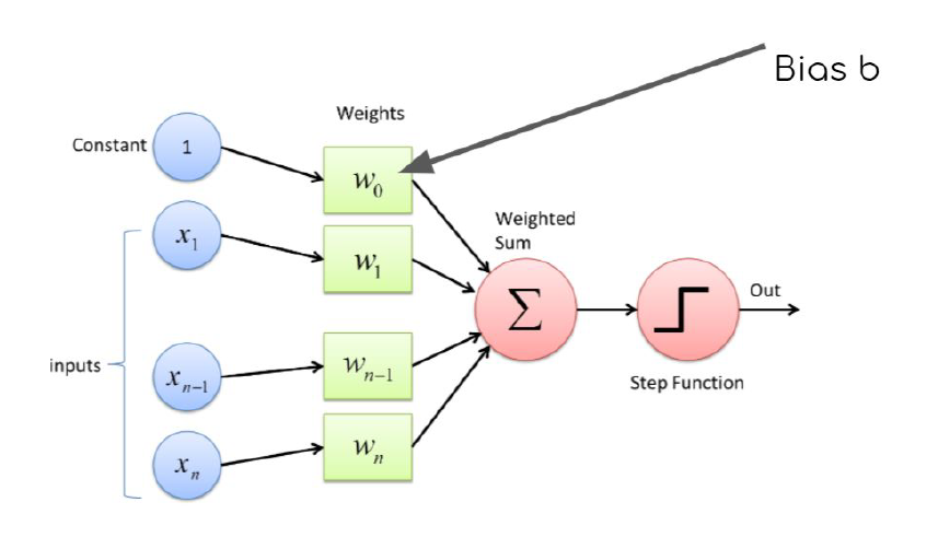
The bias term represents the inherent offset in the output when all inputs are zero. By defining \(w_0 = b\) and \(x_0=1\), we effectively transform the affine function into a linear function by augmenting the data with an additional dimension.
Perceptron Learning Algorithm
It is a supervised learning algorithm. Suppose we are given a training dataset \(\{(\mathbf{x}_i, t_i)\}_{i=1}^N\), where \(\mathbf{x}_i \in \mathbb{R}^D\) and \(t_i \in \{-1,1\}\). Let \(k\) represent the number of updates.
-
Initialize \(k \leftarrow 0\) and \(\mathbf{w}_k = \mathbf{0}\). Here \(\mathbf{w}_k \in \mathbb{R}^{D+1}\) includes the bias term. Also, \(\mathbf{x}_i \in \mathbb{R}^{D+1}\), extended by appending a constant 1.
-
While there exists an index \(i \in \{1,2,\dots, N\}\) such that \(t_i(\mathbf{w}_k^\top \mathbf{x}_i) \leq 0\), update
\[\begin{align*} \mathbf{w}_{k+1} & = \mathbf{w}_k + t_i \mathbf{x}_i \\ k & \leftarrow k+1 \end{align*}\]The condition \(t_i(\mathbf{w}_k^\top \mathbf{x}_i) \leq 0\) checks for any misclassification, ensuring that the predicted label and the ground truth have the same sign. While there exists a misclassification, we perform the above updates.
If the current \(\mathbf{w}_k\) misclassifies any data point, an update is performed using: \(\mathbf{w}_{k+1} = \mathbf{w}_k + t_i \mathbf{x}_i\). What does this update do?
Geometric Interpretation
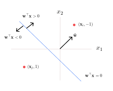
We express the model as: \(\mathbf{w}_k^\top \mathbf{x}_i = \mathbf{\tilde{w}}_k^\top \mathbf{x}_i + w_0\), where
-
\(\mathbf{w} = (w_0, w_1, \dots, w_D)\) and \(\mathbf{x} \in \mathbf{R}^{D+1}\) on the left-hand side.
-
\(\mathbf{\tilde{w}} = (w_1, \dots, w_D)\) and \(\mathbf{x} \in \mathbf{R}^D\) on the right-hand side.
The decision boundary, defined by \(\mathbf{w}_k^\top \mathbf{x}_i = 0\) (the blue line), is always perpendicular to \(\mathbf{\tilde{w}}_k\), while the bias term \(w_0\) determines its displacement from the origin.
Case 1: A Misclassified Point on the Right
Consider a misclassified point \(\mathbf{x}_i\) with the true label \(t_i=-1\) located on the right side of the decision boundary. Since the learned weights yield \(\mathbf{w}_k^\top \mathbf{x} >0\), we have \(t_i(\mathbf{w}_k^\top \mathbf{x}_i) < 0\), indicating misclassification.
The update step is performed as follows:
-
Multiply \(\mathbf{x}_i\) by \(t_i\), which, in this case, results in \(-\mathbf{x}_i\) (since \(t_i=-1\)). Note here \(\mathbf{x}_i \in \mathbb{R}^2\).
-
Add the vector \(-\mathbf{x}_i\) to \(\mathbf{\tilde{w}}_k\), yielding \(\mathbf{\tilde{w}}_{k+1}\).
-
Update the intercept term \(w_{0,k}\) to \(w_{0,k+1} = w_{0,k} + (t_i* 1) = w_{0,k} -1\).
-
Adjust the decision boundary to remain orthogonal to \(\mathbf{\tilde{w}}_{k+1}\).
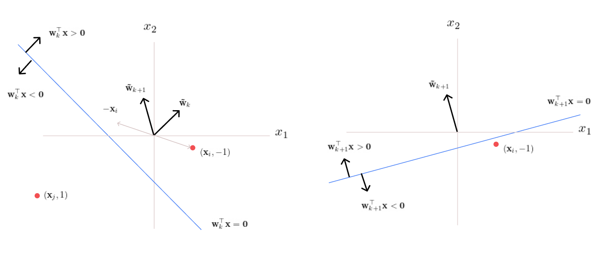
Case 2: A Misclassified Point on the Left
Now consider a misclassified point \(\mathbf{x}_j\) with the true label \(t_i=1\), located on the left side of the decision boundary. Since the learned weights yield \(\mathbf{w}_k^\top \mathbf{x} < 0\), we have \(t_i(\mathbf{w}_k^\top \mathbf{x}_i) < 0\), indicating misclassification. The same update rule is applied to correct this.
With each update, the decision boundary is adjusted to correct misclassifications. This process is repeated for every misclassified data point.
Mathematical Analysis
The misclassification condition is given by: \(t_i(\mathbf{w}_k^\top \mathbf{x}_i) \leq 0\).
Case 1: When \(t_i = 1\)
If \(\mathbf{w}_k^\top \mathbf{x}_i \leq 0\), the update equation is
Here, a positive quantity \(\|\mathbf{x}_i\|^2\) is added to \(\mathbf{w}_k^\top \mathbf{x}_i\). If this quantity is sufficiently large, \(\mathbf{w}_{k+1}^\top \mathbf{x}_i\) becomes positive. Thus adjusting the decision boundary to correct the misclassification.
Case 2: When \(t_i = -1\)
If \(\mathbf{w}_k^\top \mathbf{x}_i \geq 0\), the update equation is
Here, a positive quantity \(\|\mathbf{x}_i\|^2\) is subtracted from \(\mathbf{w}_k^\top \mathbf{x}_i\). If large enough, this forces \(\mathbf{w}_{k+1}^\top \mathbf{x}_i\) to become negative, thereby correcting the misclassification.
Convergence
For a linearly separable dataset, the Perceptron Learning Algorithm will converge in a finite number of updates. That is, if a linear decision boundary exists that achieves 100% classification accuracy, the algorithm is guaranteed to find it within a finite number of updates.
|
Note
|
Here one update refers to selecting a misclassified data point and adjusting the decision boundary accordingly. |
Convergence Criteria:
In practice, we consider the algorithm to have converged when any of the following conditions are met:
-
100% training accuracy is achieved. If multiple linear boundaries exist that provide perfect classification, the Perceptron Learning Algorithm treats them as equivalent and returns any one of them.
-
The maximum number of updates is reached.
-
The weight updates become negligible, i.e., when the difference \(\| \mathbf{w}_{k+1} - \mathbf{w}_k \|\) is very small \(< \epsilon\) for all misclassified \(\mathbf{x}_i\).
Factors Affecting Convergence:
The number of updates \(k\) and thus the speed of convergence depends on:
-
The margin \(\gamma\) between the positive and negtive class data points.
-
The distribution of data points, particularly how far they are from the origin. This is characterized by the radius \(R\) of the smallest circle that encompasses all data points.
For linearly separable data, it can be shown that the number of updates satisfies the bound: \(k < \frac{R^2}{\gamma^2}\). The Perceptron Learning Algorithm performs at most \(\frac{R^2}{\gamma^2}\) updates before finding a separating hyperplane.
Conclusion
The Perceptron learning algorithm updates its weights iteratively to correctly classify all data points. Each update repositions the decision boundary, ensuring it aligns with the true class labels. While convergence is guaranteed for linearly separable data, in non-separable cases, the algorithm continues indefinitely unless a stopping criterion is introduced.
References
-
McCulloch-Pitts neurons. (n.d.). https://mind.ilstu.edu/curriculum/mcp_neurons/index.html
-
Nielsen, M. A. (2015). Neural networks and deep learning. http://neuralnetworksanddeeplearning.com/chap1.html
-
Shivaram Kalyanakrishnan. (2017). The Perceptron Learning Algorithm and its Convergence. https://www.cse.iitb.ac.in/~shivaram/teaching/old/cs344+386-s2017/resources/classnote-1.pdf